Using Python to Visualize CTE Risk

Feb 1, 2024

Unfortunately, brain injuries and the chronic degenerative diseases that often come from them are woefully misunderstood by the general public, even as concerns about player safety and delaying the age of tackle football come more and more into the modern zeitgeist.

The motivation of this post is to augment, specify, and possibly correct our current belief systems with data obtained through Monte Carlo simulation. This type of simulation proves great for this purpose - we are not trying to publish extremely rigorous research, nor are we going to run little kids through the wringer to measure the effects of brain injury on their future development. Instead, we are going to use our common sense, a little bit of statisics, and some simple data visualization to put the risks of brain injury into the realm of “easily understandable”.

Skip down to the next blue text if you don't care about the intricacies of Monte Carlo Simulation

First, what is Monte Carlo simulation? It is a way of gaining insights from real world events by specifying models that imitate these situations and running them through many, many trials. One way to understand this is as such: suppose you have a fair coin with heads and tails, and you (somehow) don’t know what the probability of heads and tails is given a completely random flip. You could approach the true probability given enough trials. That is, you flip your perfectly fair coin one thousand, one million, approaching an infinite amount of times, to eventually obtain a fifty percent chance of either heads or tails. Frankly, this is a trivial example and is not particularly enlightening nor interesting.

However, the true beauty of Monte Carlo simulation comes from messy problems that are difficult to abstract.

Going back to the real world, the perfect game that comes to mind is poker. Say you have a given hand at a table with n people all with different personalities and skillsets. Modern theory dictates that your ability to succeed in a given situation is based on how closely you can approximate the Game Theory Optimal outcome while knowing when to deviate to gain outsized profits based on your reads. Thus, while GTO play is not the end all be all, it is the foundation of high level, modern play.

Game Theory Optimal outcomes are derived entirely from the realm of computerized mathematical analysis, in which Monte Carlo simulation is one of the oldest and best known tools used to tackle a variety of problems (although compared to modern techniques, it’s admittedly pretty clunky). One way to think about our current understanding of GTO is that we threw every tool in the book at every possible hand for every possible situation, recording how well each permutation does. Evidently, this paints a much better picture regarding the true probability you win a given hand, much more so than counting your outs or other simplified heuristics.

The question that most players are constantly trying to answer is simply: which play truly maxmizes the quantity of arbitrary variable (eg: profits, happiness, glory, etc.) in a given situation? And the way that we have managed to reveal a bit of this truth has been through tools such as Monte Carlo methods (and its much cleverer cousins).

Skip to here if you don't care about the intricacies of Monte Carlo Simulation

Okay. So what does any of this have to do with brain injuries? Simply put, we can create a model that imitates how a typical (not average) person may experience brain injuries over their lifetime. We will use a “model first, inference later” thought process, which just means that we make sure whatever we code represents reality the best it can before we try to gain insights from it. To do so, we will test our outcomes against a variety of statistics such as the average amount of force experienced by a linebacker per season, or the number of car crashes a given person gets into in their lifetimes. If we really wanted to, we could also use a market sizing approach.

After this baseline is established, this is where things start to get more interesting. We can adjust our model along a number of dimensions such as gender, sport/position played, length of career, level of play, risk preferences, and much, more. Thus, it will be flexible, allowing us to adjust based on the sorts of insights we want to glean.

A pretty natural place to start would be to define a few time series in Python. Since we now know that CTE risk is highly correlated with total force exposure over time, we’d likely want to record the total force accumulated in one time series. The other time series would simply show the severity of each impact. The motivations for including both are extremely strong. CTE is a morbid, cruel disease with severe ethical implications for how all sports should be conducted in modern society. Tracking the force of each impact is also imperative as there is a threshold for which isolated impacts can cause instant death or an increased risk for devastating diseases such as Multiple Sclerosis, Parkinson’s, Alzheimer’s, and more.

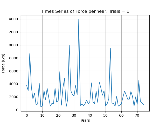
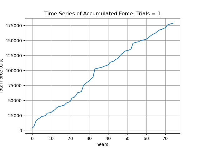
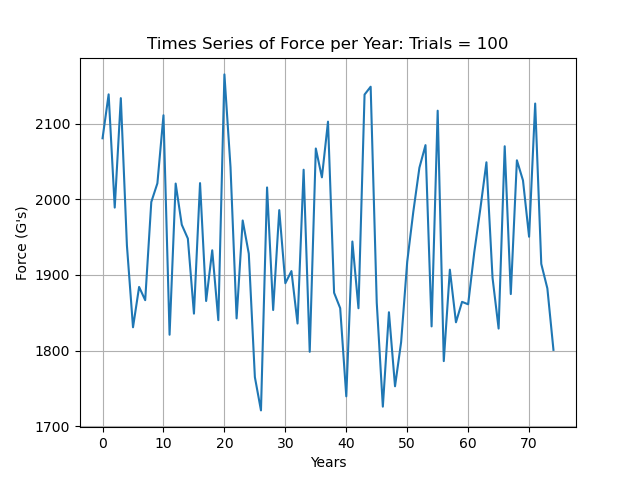
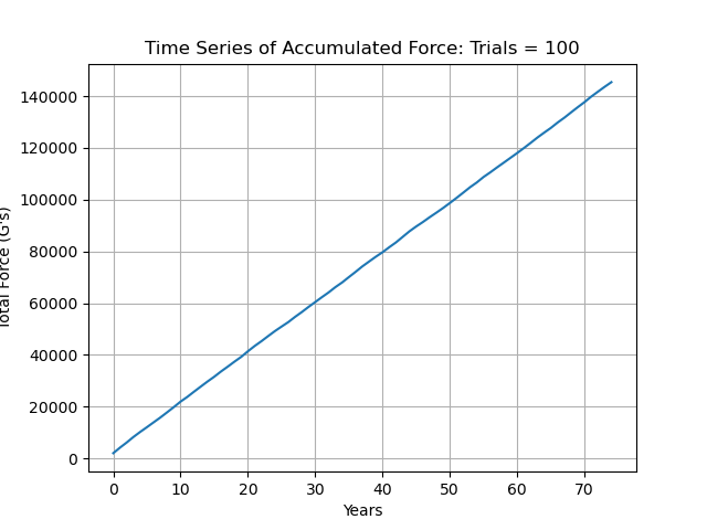
The reason that these are Monte Carlo simulations is as follows: for the number of simulations, there are individual time series generated which are summed element wise in an array that holds all of the values from all of the simulations, which is then divided by num_simulations. We can see that this process smooths out a lot of variation, especially looking at the Total Force Accumulated for fewer simulations.

For this application, I’ve also chosen for the magnitudes of the force to be lognormally distributed rather than normally distributed. This is because force experienced can never be negative. Furthermore, the population probability density function of force experienced is likely skewed right due to the inherent nature of brain injuries and head impacts. In simple terms, most people probably don’t accumulate that much force to their brain in their lifetimes, but unfortunately there are some that experience really high magnitudes (think NFL players or former combat veterans).

def simulate_time_series(num_simulations, num_intervals, mean_force, force_std):
    # These are the arrays that each simulated series is going to get added to element-wise
    monte_carlo_time_series = np.zeros(num_intervals)
    monte_carlo_total_force = np.zeros(num_intervals)

    for i in range(0, num_simulations):
        # These are the placeholder arrays for each run of the simulation
        sample_time_series = np.zeros(num_intervals)
        sample_total_force = np.zeros(num_intervals)

        for j in range(0, num_intervals):
            random_force = np.random.lognormal(mean_force, force_std)

            # If the model is changed back to a normal distribution with possibility of the sample variable taking on negative values, then all values are counted as non-negative real numbers.
            if random_force < 0:
                random_force = 0

            sample_time_series[j] = random_force
            sample_total_force[j] = random_force + sample_total_force[j - 1]

        monte_carlo_time_series += sample_time_series
        monte_carlo_total_force += sample_total_force

    # This is to scale down the array because it will have the sum of n = num_simulations sample variables at each element
    monte_carlo_time_series = monte_carlo_time_series / num_simulations
    monte_carlo_total_force = monte_carlo_total_force / num_simulations
    return (monte_carlo_time_series, monte_carlo_total_force)

def main():
    # ...
    mean_force = np.random.normal(7, 1)
    force_std = np.random.normal(1, 1)
    monte_carlo_time_series, monte_carlo_total_force = simulate_time_series(num_simulations, years, mean_force, force_std)
    # ...

However, these simulations are pretty far off the mark. First, since we have defined our interval for the time series as a year, we would not expect nearly as much variation as we are seeing. Unless you go from living on planet Earth to being on the International Space Station (or vice versa), you would likely not see the severe drop offs or increases in force per year that we see in both cases.

Another thing that we have failed to account for is the fact that generally force per year is higher for some time periods of our lives. When we are children or adolescents, we’re naturally more mobile and most people will thus accumulate more force during these time periods. The average age of NFL players is 26.4 years old, and the average length of their careers are about three years. So to not have these realities included in our model would be a disservice to the things that we are trying to capture.

Similarly, forces above certain thresholds affect different demographics more than others. The biology of younger children is entirely different from fully developed adults, making them much more susceptible to forces of the same magnitude. Women, while less likely to accumulate as much force as men over their lifetimes, may have a higher risk of developing adverse conditions from less force exposure. Older people get more susceptible to TBI as time passes and heal more slowly from them as they age. These realities are much harder to include into our model but are important and should be mentioned.

To start, we can define a function that has higher values around adolescense and early adulthood and tapers off past those ages. We will use this to scale our random forces inside our for-loops, and we will also adjust the mean and standard deviation that we pass into our method to decrease variance to a reasonable level.